Personal project / Spatial databases / 2024

City Transport Study.
Greater Melbourne, mapped.

I used PostgreSQL and PostGIS to bring transport schedules and geographic boundaries together, compare stop density and explore how public transport coverage varies across Greater Melbourne.

PostgreSQLPostGISSQLGTFSDBeaverGDAL / ogr2ogr

Read the project report Download report

8.1 millionImported stop-time records*

3 transport modesTrain, tram and bus

Spatial SQLFrom raw tables to mapped comparisons

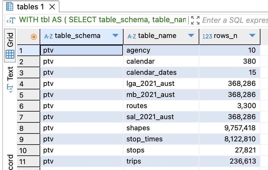
*Row count from the imported GTFS source table, before Greater Melbourne filtering. It is not a count of passenger journeys.

The approach

Make the data connect.

The project combines PTV GTFS schedules with ABS geographic boundaries. I prepared the database, linked related transport tables, and used spatial queries to compare service provision across SA3 statistical areas.

01 / PREPARE

Restore and inspect

Load GTFS into PostgreSQL, import boundary geometries with ogr2ogr, and inspect tables and row counts in DBeaver.

02 / QUERY

Join and classify

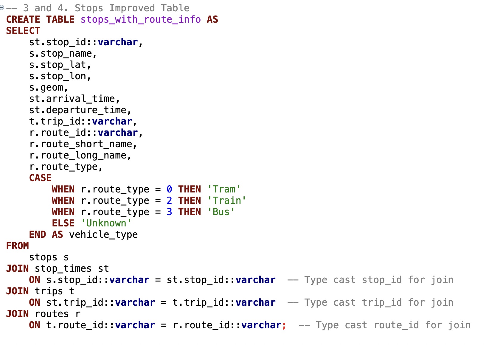
Connect stops, stop times, trips and routes with SQL joins. Use CASE expressions, CTEs and aggregation to organise the analysis.

03 / MAP

Compare spatial patterns

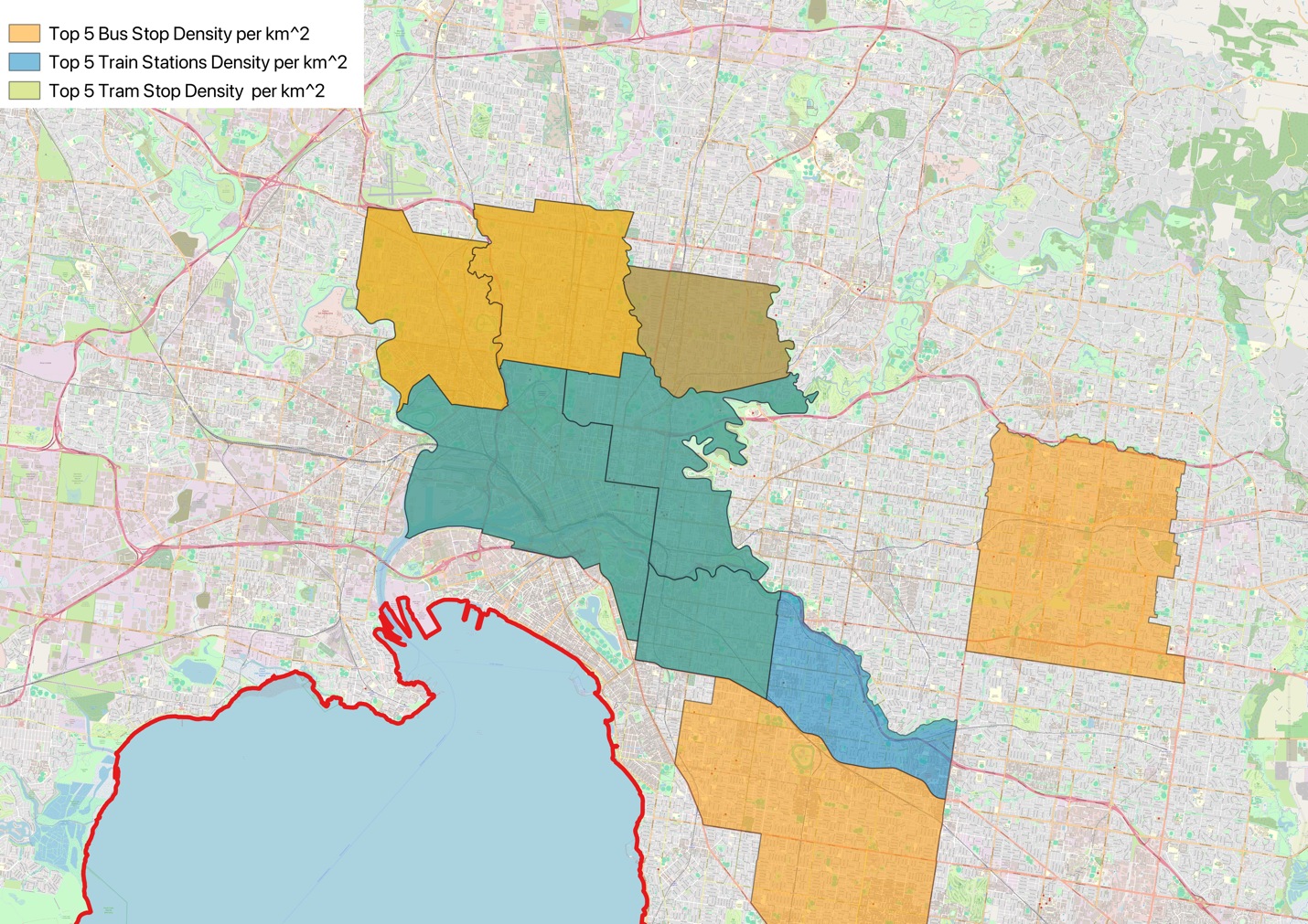
Build geographic tables with PostGIS, compare stops per square kilometre and rank areas by transport mode.

Evidence from the work

Original maps. Real database outputs.

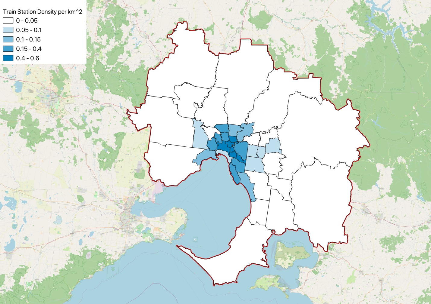
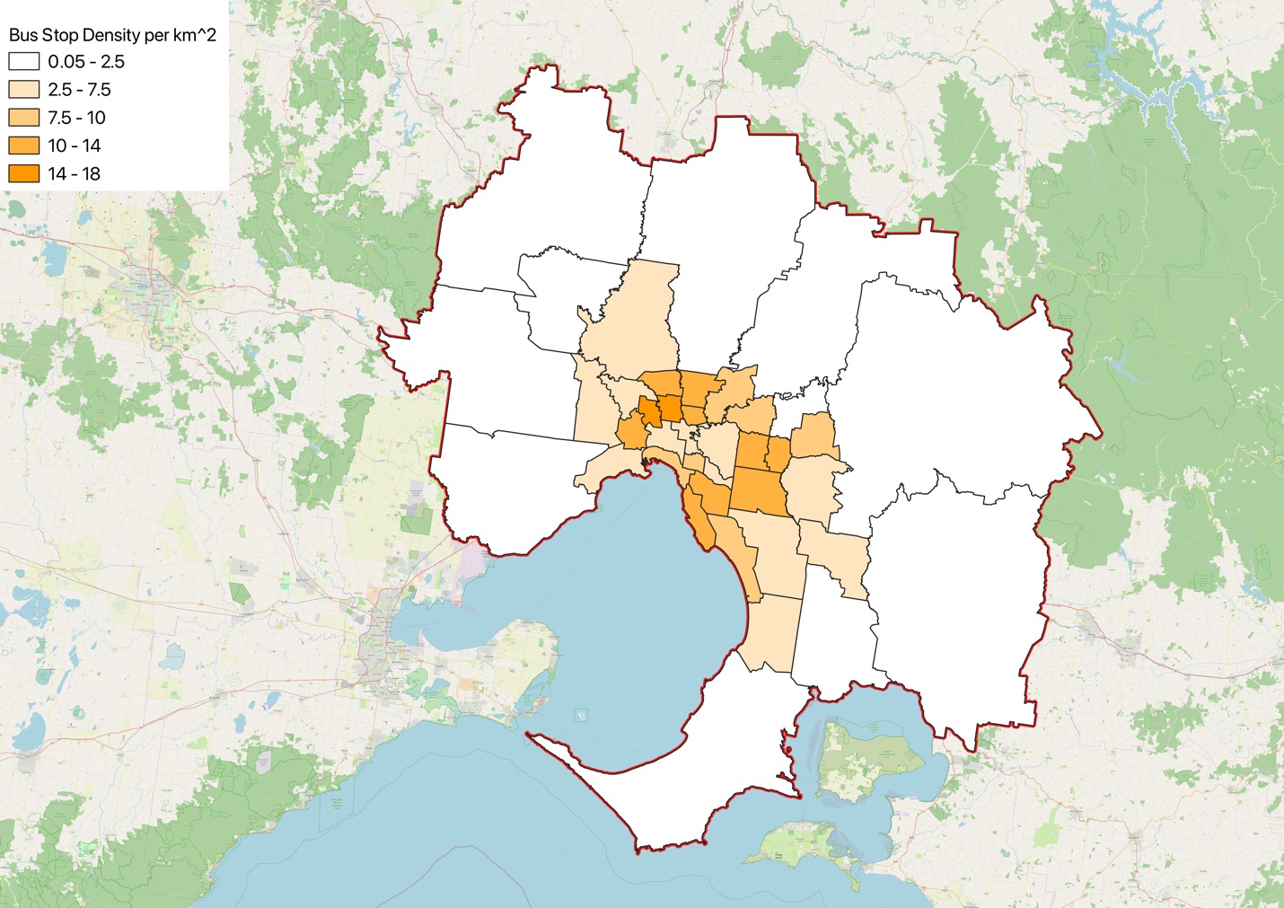
These figures are taken directly from my report. Open any image for a closer look.

Choropleth map of train station density per square kilometre across Greater Melbourne — **Train station density**Spatial aggregation and a density-based comparison of rail coverage.

Choropleth map of bus stop density per square kilometre across Greater Melbourne — **Bus stop density**A comparison with the bus network’s broader geographic footprint.

Map highlighting overlaps among the five areas with highest train, tram and bus stop density — **Where transport modes overlap**Comparing the top five areas for each mode shows how the ranking changes and where high-density networks overlap.

DBeaver query output showing imported PostgreSQL tables including 8,122,810 stop-time records — **Working with substantial source tables**Database outputs document the imported GTFS tables and their record counts.

SQL statement joining stops, stop times, trips and routes and classifying vehicle types with CASE — **Relational SQL in practice**Multi-table joins and conditional classification prepare the transport data for analysis.

What I took from it

Good analysis needs clear assumptions.

The density maps show stronger rail and tram concentration around inner Melbourne, with bus stops providing a broader footprint. Comparing the modes shows why a single network-wide measure can hide local differences.

How to read the results

The SQL groups SA3 statistical areas; the original report labels these as LGAs.
Stop density is one measure of coverage. It does not account for population, ridership or actual delays.
The exploratory catchment buffers require recalculation in a projected coordinate system before validating 400 m / 800 m distances.
Counting six departures in an hour does not prove evenly spaced ten-minute service.

Data sources: PTV GTFS and ABS digital boundary files. The downloadable report retains the analysis, figures, source references and SQL appendix, with clarifications on its new cover. Technical reference: PostGIS buffer distance units.

Let’s talk about the work

Data skills.
Practical application.

Interested in my approach to databases, reporting or business operations? I’d be glad to walk you through it.

Get in touch ↗Explore my other work →

City Transport Study.Greater Melbourne, mapped.